Classifying breast tumours from 19,644 genes, and finding the few that matter

Context

Breast cancer is treated according to a handful of labels. The PAM50 molecular subtype comes from gene expression by definition. The hormone-receptor group, meaning ER, PR and HER2 status, is a pathology-lab result, and the histological type, ductal or lobular, comes from a pathologist reading a slide. My dissertation, titled "Discovery of Potent Prognostic Biomarkers in Cancer", asked how much of those last two labels the expression data carries anyway, and which genes carry it. As far as I could find, nobody had tried to predict histological type from RNA-seq, so that was the target I cared about most.

The data was SCAN-B, a Swedish cohort of 3,207 primary breast tumours with bulk RNA-seq over 19,644 genes and clinical annotations, public on GEO as GSE202203↗. It is a wide, short matrix, with six times more features than samples. The classes are badly unbalanced, 90 Normal-like tumours against 1,232 Luminal A at one extreme, and roughly one lobular tumour for every seven ductal. Several clinical fields had holes, including 2,057 tumours with no Ki-67 value. The budget was one summer, one laptop and no GPU.

Approach

The first thing I did with the data was reproduce a result from the paper that published it, the Spearman correlation between ESR1 and ESR2, and got the same figure of -0.24. That was the check that the parsing was right before anything was built on it.

Every target then went through the same pipeline. Parse the two GEO series-matrix files into a clean clinical table. Fill the 154 missing receptor groups with the mode, cap outliers, and drop the classes that were not a label at all: "Unclassified" for PAM50 and "Other" for histology, which made histology a two-class problem. Split 80/20, stratified. Oversample the minority classes with SMOTE and standardise, both fitted on the training fold only. Models ran on TPM; differential expression ran on the raw counts.

Then the part that mattered, laid out in Figure 1. Six ways of choosing features and four classifiers, twenty-four combinations per target, every one tuned by randomised search under five-fold cross-validation. The selectors ran from univariate ANOVA ranking with a swept k, through PCA and the genes that load most on its top components, to the twenty and fifty most differentially expressed genes from DESeq2 in R, and finally linear discriminant analysis. The classifiers were logistic regression, a linear-kernel SVM, random forest and k-nearest neighbours.

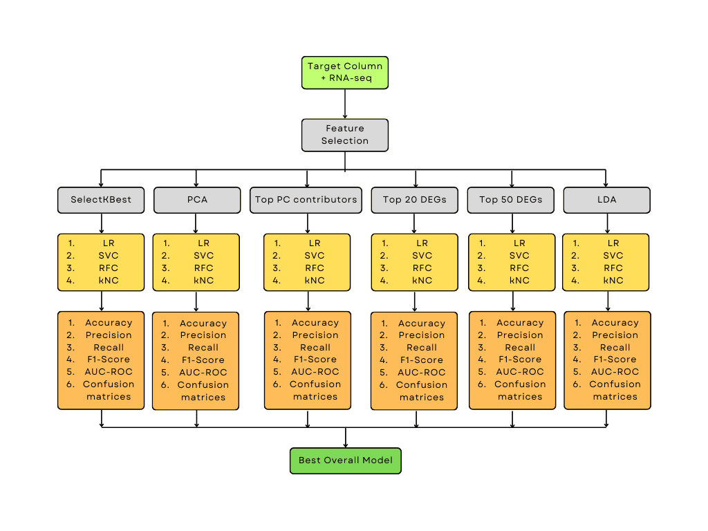
Held-out test sets of roughly 600 tumours gave the final numbers. Accuracy was reported but never trusted on its own. Macro F1, per-class recall and one-vs-rest AUC decided between models, because the classes I cared about most were the small ones.

A few things were tried and dropped before any of that: a Keras MLP tuned with keras-tuner, k-means clustering, XGBoost at 0.798 on PAM50, and mRMR feature selection, which crashed. The first of those is the first decision below.

Decisions

[01]Design decisionClassical models, no neural network

Decision

A tuned multilayer perceptron was built, evaluated and left out of the final comparison.

Why

It reached 80.0% test accuracy on PAM50 after tuning, below its own untuned run at 80.3%. The linear SVM in the final pipeline reached 90.3%. The two runs did not share identical features, but the gap was not going to close: with about 2,500 training rows and 19,000 features there was nothing for depth to learn that a linear boundary on well-chosen genes did not.

Tradeoff

The write-up has no deep-learning chapter, which some readers expect from a 2024 ML dissertation. The numbers did not support one.

[02]Design decisionPick the model on minority recall, not accuracy

Decision

For PAM50 the linear SVM was chosen over random forest despite the forest's slightly higher cross-validated accuracy, 0.910 against 0.901. For histology the choice went the same way.

Why

The SVM recalled the rare classes far better: 0.73 against 0.55 on Normal-like tumours, 0.71 against 0.55 on lobular. Macro F1 on histology was 0.86 against 0.81. A classifier that misses the rare subtype is no use in a clinic, whatever its headline accuracy.

Tradeoff

A linear SVM has no native feature importance, so finding the genes meant permutation importance, which is slow and noisy.

[03]Design decisionA different feature selector for each target

Decision

Univariate selection with k re-tuned per target for PAM50 (k = 390) and receptor group (k = 130); the top fifty DESeq2 genes for histology.

Why

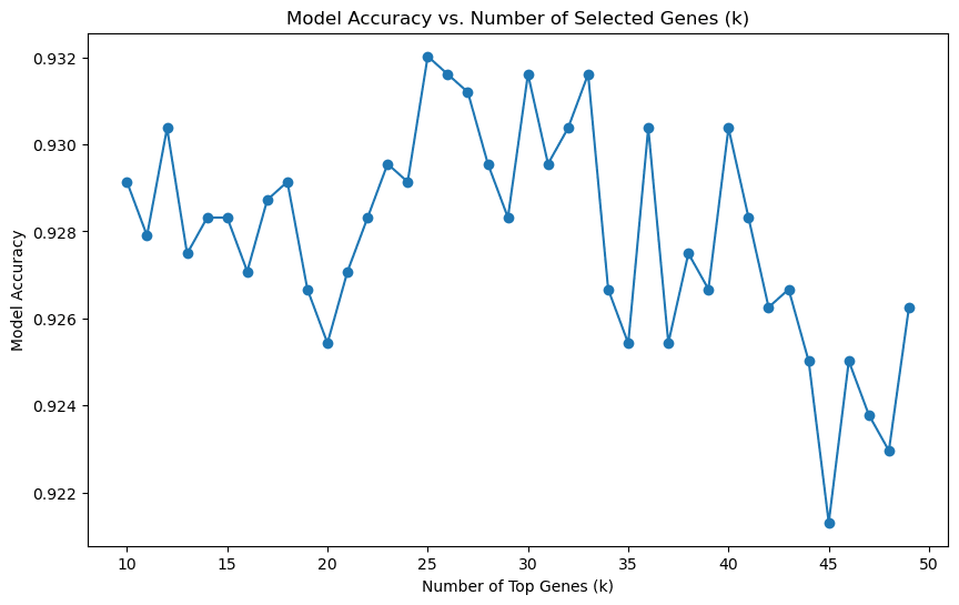
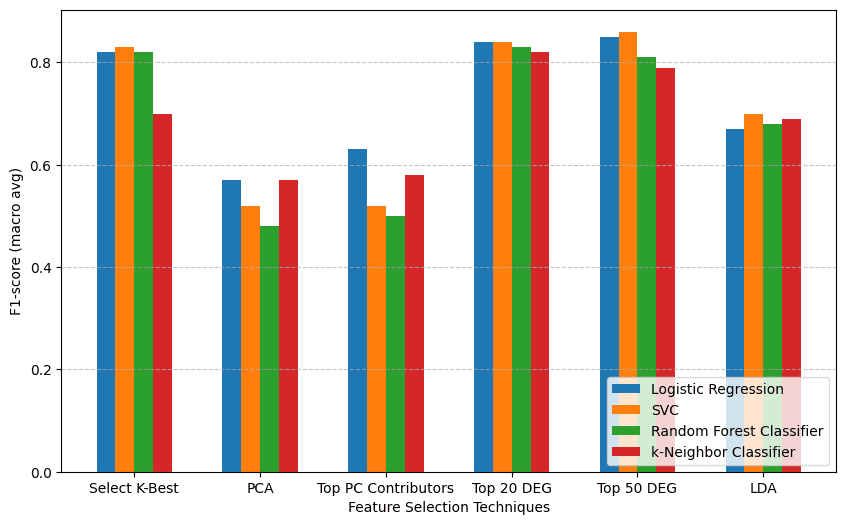
Each target had a different sweet spot. For histology, sweeping k from 10 to 50 gave the noisy plateau in Figure 2, hovering around 0.93 with no trend. The fifty-gene DESeq2 list scored 0.938 cross-validated with the SVM. Figure 3 shows the wider pattern: the two DESeq2 lists lead for every classifier, top-50 ahead for logistic regression and the SVM, top-20 ahead for random forest and k-nearest neighbours. A gene list is also something a biologist can read, which a value of k is not.

Tradeoff

Gene lists crossed from R to Python by hand, and k = 390 sat on a plateau where 350 or 450 would have done as well. Three pipelines are more to maintain than one.

[04]Design decisionOversample the minorities partway, not to parity

Decision

SMOTE on the training fold only, raising the minority classes to 253, 256 and 350 examples rather than matching the majority.

Why

The counts came from trial and error, and I said so in the dissertation. The point of oversampling was recall on the rare classes, and that is what the trials were judged on.

Tradeoff

HER2 and Normal-like stayed the hardest PAM50 classes, with test recall of 0.80 and 0.73. For lymph-node status SMOTE was switched off altogether, and the model still could not beat the majority class.

[05]Design decisionReport the failures

Decision

Tumour size and lymph-node status were the original targets. Both were dropped from the headline results and written up as negative findings.

Why

The best lymph-node model scored 0.628 against a majority-class baseline of 0.625. The best tumour-size model scored 0.707 against 0.654, with zero recall on the largest tumours. Side experiments on age group, tumour grade, a regression on tumour size and a Cox survival model fared no better, at 0.44, 0.68, an R² of 0.05 and a concordance index of 0.65. Bulk expression does not carry that information, and saying so is a result.

Tradeoff

The pivot happened after those results were in, so the negatives went into the dissertation as prose rather than tables, and the side experiments not at all. Both examiners graded it A+, and both made the same criticism: the null results deserved their own numbers.

Results

Logistic regression on the same features scored 0.890, 0.909 and 0.938, so the gain from model choice was small and the gain from feature choice was large. PCA was the worst feature set for every target, which Figure 3 shows for histology, bottoming out at 0.622 for k-nearest neighbours on PAM50. One-vs-rest AUC was 0.98 or better for every PAM50 class, 0.92 to 0.99 across the receptor groups, and 0.94 for lobular against ductal. The confusions were the ones a pathologist would predict: Luminal A against Luminal B, and HER2-positive against HER2-negative within the ER-positive group.

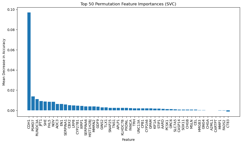
Then the genes. Permutation importance on the histology SVM put CDH1 first by a wide margin, as Figure 4 shows: shuffling it cost about 0.10 of accuracy, roughly seven times the next gene. CDH1 encodes E-cadherin, and losing it is the textbook marker of lobular carcinoma. DESeq2 agreed, ranking CDH1 the most significant gene between the two types by a long way. The model had rediscovered the pathology from the expression data, which was the check that made the rest of the gene lists worth reading.

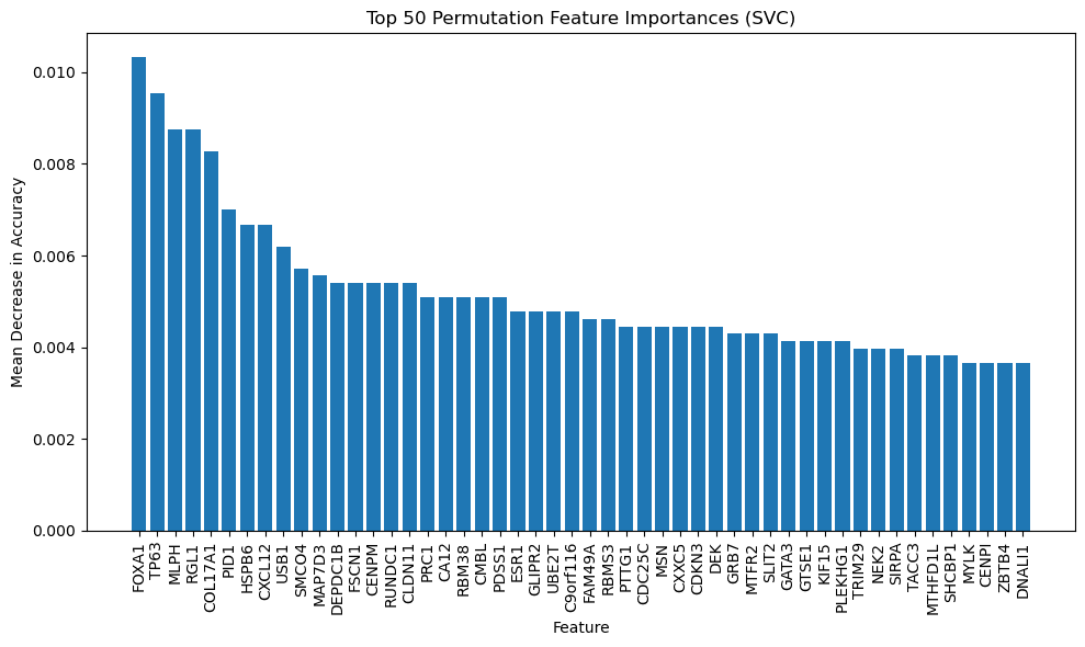
PAM50 looked nothing like that. In Figure 5 the importances slope down gently from FOXA1, TP63 and MLPH, with no gene above 0.011. That is what you would expect of a label that is itself defined by fifty genes. The three classifiers agreed on only two genes across their top-fifty lists.

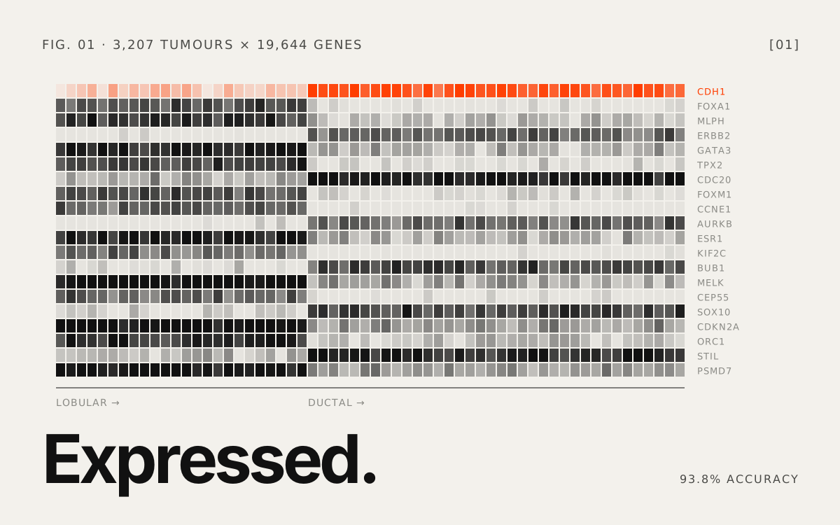
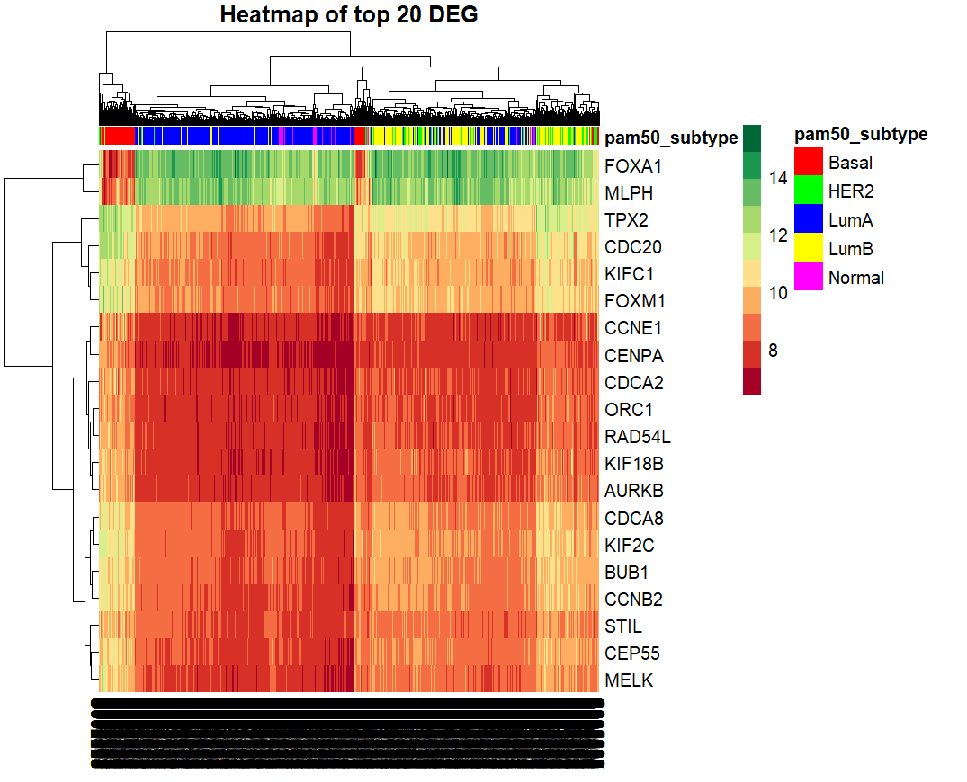
The differential-expression view of PAM50 is Figure 6: the twenty most significant genes, clustered across the whole cohort. The clustering splits the tumours by proliferation rather than by subtype name. One block is almost entirely Luminal A and Normal-like, with the cell-cycle genes low. The other holds Luminal B, HER2 and Basal, with the same genes high. FOXA1 and MLPH stay high almost everywhere and fall only in the Basal stripes. Across the three targets the lists put ERBB2, GATA3, SOX10, CDKN2A and CDH1 forward as the candidates worth a clinician's time, which the dissertation left as future work.

Looking back

I found a leak in my own pipeline. Linear discriminant analysis as a feature selector gave cross-validated accuracies of 0.95 to 0.97 and test accuracies of 0.80 to 0.88. The LDA had been fitted on the whole training set before cross-validation, so every fold had already seen its validation rows through the projection. The test numbers stand, because the test set never touched it, and LDA lost anyway. But that row's cross-validation column was wrong, and it is the reason a selector belongs inside the pipeline the search wraps, never outside it.

The expensive experiments were the cheap ones. The MLP, XGBoost, mRMR and clustering took about a month, from late July to late August, and contributed nothing to the result except confidence that the linear model was right. That confidence was worth the time. Leaving them out of the write-up was not.

The code has the gaps of a solo summer project. The random forest ran without a fixed seed. Thirty of every hundred logistic-regression fits in the search failed on invalid solver and penalty pairs. The saved models did not include their scaler or selector. Tracking my changes and pinning my library versions from day one would have caught some of that, and I would not skip them again.

What else I would change. More time on feature selection, which I also wrote in the dissertation. A second cohort to validate on, since every number here is one dataset and one split. And a pathologist in the room early, because the gene lists raised questions only a clinician could answer.